Difference between revisions of "Tools1D"
| (5 intermediate revisions by the same user not shown) | |||
| Line 1: | Line 1: | ||
[[File:Tools1D.png|600px]] | [[File:Tools1D.png|600px]] | ||
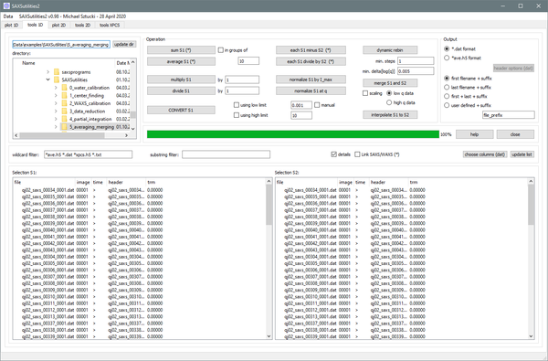
| − | Graphical user interface for typical operations on one-dimensional files in ASCII (general) or HDF5 format (ID02) like summing, averaging, subtraction, merging, ... Routines for data conversion are available. | + | Graphical user interface for typical operations on one-dimensional files in ASCII (general) or HDF5 format (ID02: ending on _ave.h5 or _xpcs.h5) like summing, averaging, subtraction, merging, ... Routines for data conversion are available. |
=== Features: === | === Features: === | ||
* Data sets with q vector, data and optionally error are supported. An appropriate error proagation is implemented for all available operations. | * Data sets with q vector, data and optionally error are supported. An appropriate error proagation is implemented for all available operations. | ||
| + | * Data are automatically interpolated to the q scale of the first file provided (if necessary). | ||
| + | * Combines SAXS/WAXS measurements can be now treated simultaneously. The same operation is executed for SAXS and WAXS files individually. | ||
* History of performed operations is saved either in the first header line (ASCII) or and appropriate header key (HDF5). | * History of performed operations is saved either in the first header line (ASCII) or and appropriate header key (HDF5). | ||
| + | * Output file name and data format can be chosen. | ||
| + | * A conversion between ASCII (*.dat) and HDF5 (*ave.h5) is available. | ||
| + | === Specific features: === | ||
| + | In the following a list of functions with more detailed description: | ||
| − | [[File:Tools1Dplot.png| | + | ==== CONVERT ==== |
| + | <hr> | ||
| + | This allows to re-write all data sets selected in Selection S1. | ||
| + | * You can optionally restrict the q range of the created files at low and high q. | ||
| + | * By activating 'manual' you can choose the low q limit for each file separately by clicking on a graph. '''This is ideal for treating data which show unwanted artefacts at low q!''' | ||
| + | * The output data format can be chosen in the right top corner of the GUI. '''This is intended for converting data from ASCII to HDF5 and inverse.''' | ||
| + | |||
| + | ==== SUM, AVERAGE, MINUS (each), DIVIDE (each) ==== | ||
| + | <hr> | ||
| + | * Summing and averaging can be done in groups of acertain number of images. The length of the selection must be a multiple of this number. | ||
| + | * All four functions can be combined with the option 'Link SAXS/WAXS'. In this case the operation is executed for two groups of files identified by _saxs_ and _waxs_ in the file name. | ||
| + | |||
| + | ==== NORMALIZE ==== | ||
| + | <hr> | ||
| + | * This functions allow to either normalize the selected files by the maximum intensity or at a selected q value. | ||
| + | * In the second case, the q value is selected graphically. '''This allows to compare curves by scaling them in intensity.''' | ||
| + | [[File:Tools1Dplot.png|400px]] | ||
| + | |||
| + | ==== DYNAMIC REBIN ==== | ||
| + | <hr> | ||
| + | This function is particularly useful for data which are plotted on a logarithmic q scale: | ||
| + | Usually, data sets have a q scale with equidistant points in a linear scale. Plotting them in a logarithmic way results in a very high density of points at high q. Typically, the high q range is also the range where the statistical error of the measured intensity is highest. | ||
| + | * '''The dynamic rebin function allows to arrange homogeneously the measured datapoints on a logarithmic q scale.''' | ||
| + | * The value of min. delta[log(q)] (typically 0.005) defines the minimum distance between datapoints on a logarithmic q scale. In case there are datapoints closer, they will get averaged. In particular, measured datapoints at high q get averaged in this way. | ||
| + | * The input min. steps defines the number of datapoints being averaged at low q. 1 means no averaging until the min. delta[log(q)] condition is reached. By increasing this value to 3 or more (must be odd) an according number of surrounding datapoints are averaged into each point, which results in a smoothing over the full q range. | ||
| + | * Do not forget to compare the result of the dynamic re-binning. | ||
| + | * '''This function is also very interesting for data fitting''' using functions with numerical integrations as it allows to reduce the number of datapoints per file and therefore the calculation time. | ||
| + | |||
| + | ==== MERGE ==== | ||
| + | <hr> | ||
| + | This function allows to merge data sets measured either with different detectors or at different sample to detector distances. | ||
| + | * The merging is done in a plot window. Two clicks define the range of an overlapping range. Within this range an average of the measured intensity of both files is calculated. Outside of it only the intensity of the one or the other data file is used. | ||
| + | * It is also possible to allow scaling of the file situated either at the high or the low q limit [scaling (low/high)] (depending if the absolute intensity level of the low or high q data are more reliably). | ||
| + | * The result of the merging is previewed and can be optimized for each pair of curves. | ||
Latest revision as of 10:12, 5 May 2020
Graphical user interface for typical operations on one-dimensional files in ASCII (general) or HDF5 format (ID02: ending on _ave.h5 or _xpcs.h5) like summing, averaging, subtraction, merging, ... Routines for data conversion are available.
Contents
Features:
- Data sets with q vector, data and optionally error are supported. An appropriate error proagation is implemented for all available operations.
- Data are automatically interpolated to the q scale of the first file provided (if necessary).
- Combines SAXS/WAXS measurements can be now treated simultaneously. The same operation is executed for SAXS and WAXS files individually.
- History of performed operations is saved either in the first header line (ASCII) or and appropriate header key (HDF5).
- Output file name and data format can be chosen.
- A conversion between ASCII (*.dat) and HDF5 (*ave.h5) is available.
Specific features:
In the following a list of functions with more detailed description:
CONVERT
This allows to re-write all data sets selected in Selection S1.
- You can optionally restrict the q range of the created files at low and high q.
- By activating 'manual' you can choose the low q limit for each file separately by clicking on a graph. This is ideal for treating data which show unwanted artefacts at low q!
- The output data format can be chosen in the right top corner of the GUI. This is intended for converting data from ASCII to HDF5 and inverse.
SUM, AVERAGE, MINUS (each), DIVIDE (each)
- Summing and averaging can be done in groups of acertain number of images. The length of the selection must be a multiple of this number.
- All four functions can be combined with the option 'Link SAXS/WAXS'. In this case the operation is executed for two groups of files identified by _saxs_ and _waxs_ in the file name.
NORMALIZE
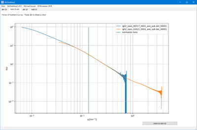
- This functions allow to either normalize the selected files by the maximum intensity or at a selected q value.
- In the second case, the q value is selected graphically. This allows to compare curves by scaling them in intensity.
DYNAMIC REBIN
This function is particularly useful for data which are plotted on a logarithmic q scale: Usually, data sets have a q scale with equidistant points in a linear scale. Plotting them in a logarithmic way results in a very high density of points at high q. Typically, the high q range is also the range where the statistical error of the measured intensity is highest.
- The dynamic rebin function allows to arrange homogeneously the measured datapoints on a logarithmic q scale.
- The value of min. delta[log(q)] (typically 0.005) defines the minimum distance between datapoints on a logarithmic q scale. In case there are datapoints closer, they will get averaged. In particular, measured datapoints at high q get averaged in this way.
- The input min. steps defines the number of datapoints being averaged at low q. 1 means no averaging until the min. delta[log(q)] condition is reached. By increasing this value to 3 or more (must be odd) an according number of surrounding datapoints are averaged into each point, which results in a smoothing over the full q range.
- Do not forget to compare the result of the dynamic re-binning.
- This function is also very interesting for data fitting using functions with numerical integrations as it allows to reduce the number of datapoints per file and therefore the calculation time.
MERGE
This function allows to merge data sets measured either with different detectors or at different sample to detector distances.
- The merging is done in a plot window. Two clicks define the range of an overlapping range. Within this range an average of the measured intensity of both files is calculated. Outside of it only the intensity of the one or the other data file is used.
- It is also possible to allow scaling of the file situated either at the high or the low q limit [scaling (low/high)] (depending if the absolute intensity level of the low or high q data are more reliably).
- The result of the merging is previewed and can be optimized for each pair of curves.

